Lecture 4: Robust Analog Circuit Sizing Under Process Variations

@luk036

2022-10-12

📝 Abstract

The lecture focuses on the robust sizing of analog circuits under process variations. It analyzes the challenges that arise when designing analog circuits at the 20nm process node, including double-patterning, layout-dependent effects, new local interconnect layers, and the use of FinFET transistors. The lecture stresses the importance of designing circuits with robustness in mind by factoring in process variations in the specification requirements. The lecture presents the concept of formulating the analog circuit sizing problem and identifies the difficulties involved, such as the high level of flexibility and susceptibility to variations. The lecture also explores various approaches to computer-aided design (CAD) for analog circuits, including knowledge-based and optimization-based techniques. The lecture discusses emerging techniques in geometric programming (GP), introducing a new method for solving robust GP problems using the affine arithmetic and the ellipsoid technique. An example of CMOS two-stage operational amplifier design demonstrates the application of the robust geometric programming approach.

🔑 Keywords

• Analog circuit 模拟电路
• Design for robustness 鲁棒性设计
• Worst-case scenarios 最坏情景
• Affine arithmetic 仿射运算
• Convex programming 凸规划
• Geometric programming 几何规划
• Posynomial 正项式 (Positive + polynomial)
• Ellipsoid method 椭球法

🗺️ Overview

• Challenges of 20nm Analog Design

• Design for variability

• Design for robustness

• Analog circuit sizing problem formulation

• Robust geometric programming

• Affine arithmetic for worst case scenarios

• Design examples

📖 Introduction

Costs 28nm 20nm

Fab Costs 3B 4B - 7B Process R&D 1.2B 2.1B - 3B Mask Costs 2M - 3M 5M - 8M Design Costs 50M - 90M 120M - 500M

: Fab, process, mask, and design costs are much higher at 20nm (IBS, May 2011)

Challenges at 20 nm

• Double-patterning aware

• Layout-dependent effects

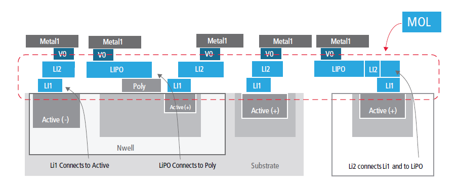
• New local interconnect layers

• >5,000 design rules

• Device variation and sensitivity

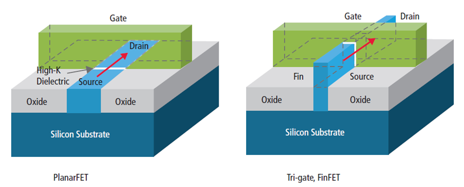
• New type of transistor - FinFET

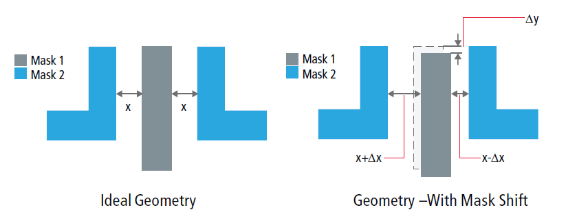
👫 Double Patterning

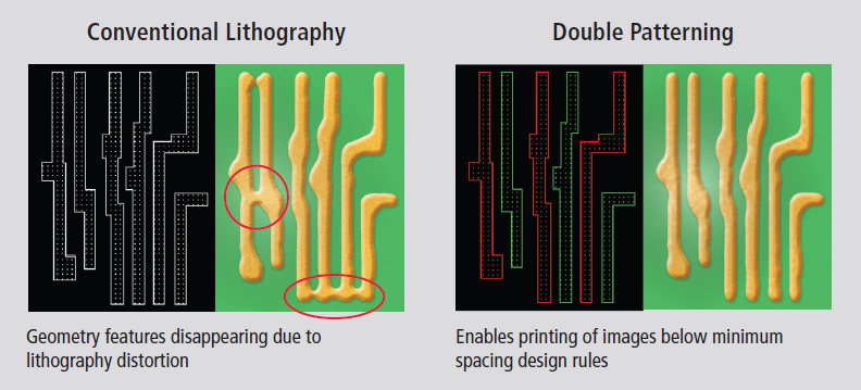
Overlay Error (Mask Shift)

• Parasitic matching becomes very challenging

  

Layout-Dependent Effects

New Local Interconnect Layers

New Transistor Type: FinFET

Design for Robustness

• Process variations must be included in the specification.

Basic Design Flow

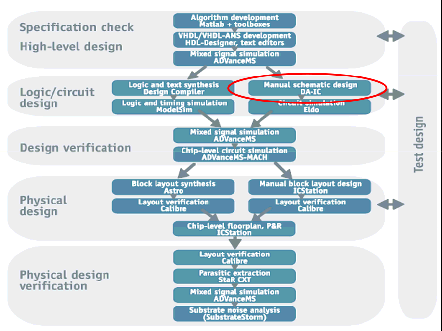
Top-down Design Phases

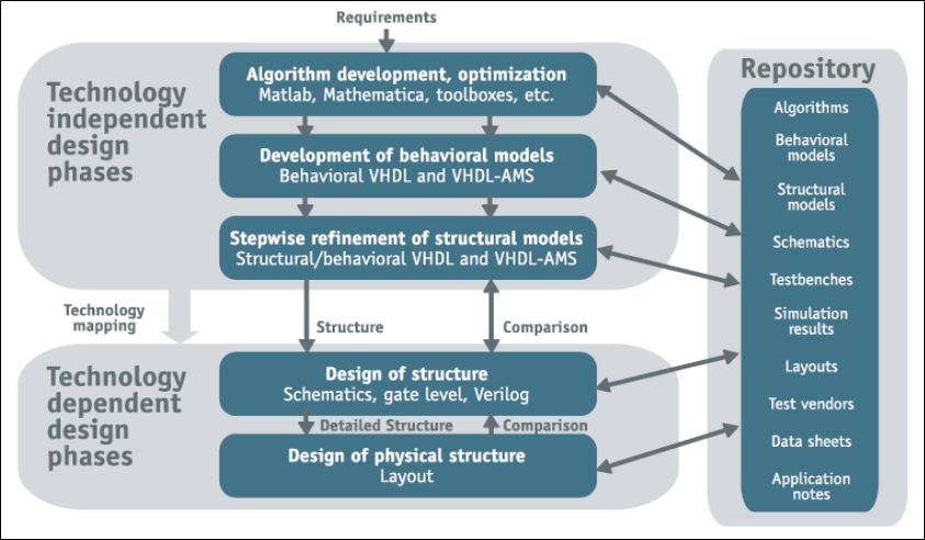
Basic Flow of Analog Synthesis

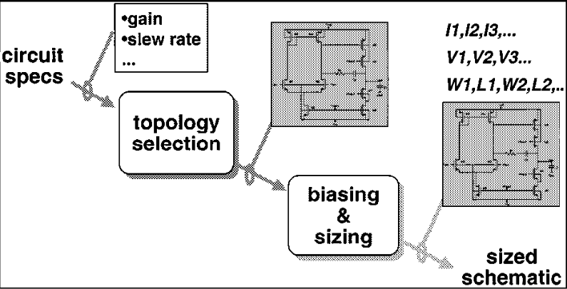
Analog Circuit Sizing Problem

• Problem definition:
  • Given a circuit topology, a set of specification requirements and technology, find the values of design variables that meet the specifications and optimize the circuit performance.
• Difficulties:
  • High degrees of freedom
  • Performance is sensitive to variations

Main Approaches in CAD

• Knowledge-based
  • Rely on circuit understanding, design heuristics
• Optimization based
  • Equation based
    • Establish circuit equations and use numerical solvers
  • Simulation based
    • Rely on circuit simulation

In practice, you mix and match of them whenever appropriate.

Geometric Programming

• In recent years, techniques of using geometric programming (GP) are emerging.
• In this lecture, we present a new idea of solving robust GP problems using ellipsoid method and affine arithmetic.

Lecture 04b - Robust Geometric Programming

Outline

• Problem Definition for Robust Analog Circuit Sizing
• Robust Geometric Programming
• Affine Arithmetic
• Example: CMOS Two-stage Op-Amp
• Numerical Result
• Conclusions

Robust Analog Circuit Sizing Problem

• Given a circuit topology and a set of specification requirements:

• Find the worst-case design variable values that meet the specification requirements and optimize circuit performance.

Robust Optimization Formulation

• Consider $$\begin{array}{ll}\text{minimize}& {\sup }_{q\in \mathbb{Q}}{f}_0(x,q),\\ \text{subject to}& f_j(x,q)\le 0\\ & \forall q\in \mathbb{Q}\text{and}j=1,2,\cdots ,m,\end{array}$$ where
  • $x\in {\mathbb{R}}^n$ represents a set of design variables (such as $L$, $W$),
  • $q$ represents a set of varying parameters (such as $T_{OX}$)
  • $f_j\le 0$ represents the $j$th specification requirement (such as phase margin $\ge 60^{\circ }$).

Geometric Programming in Standard Form

• We further assume that $f_i(x,q)$'s are convex for all $q\in \mathbb{Q}$.
• Geometric programming is an optimization problem that takes the following standard form: $$\begin{array}{lll}\text{minimize}& p_0(y)& \\ \text{subject to}& p_i(y)\le 1,& i=1,\dots ,l\\ & g_j(y)=1,& j=1,\dots ,m\\ & y_k>0,& k=1,\dots ,n,\end{array}$$ where
  • $p_i$'s are posynomial functions and $g_j$'s are monomial functions.

Posynomial and Monomial Functions

• A monomial function is simply: $$g(y)=c{y}_1^{{\alpha }_1}{y}_2^{{\alpha }_2}\cdots y_n^{{\alpha }_n},y_k>0.$$ where
  • $c$ is non-negative and ${\alpha }_k\in \mathbb{R}$.
• A posynomial function is a sum of monomial functions: $$p(y)=\sum _{s=1}^T{c}_s{y}_1^{{\alpha }_{1,s}}{y}_2^{{\alpha }_{2,s}}\cdots y_n^{{\alpha }_{n,s}},y_k>0,$$
• A monomial can also be viewed as a special case of posynomial where there is only one term of the sum.

Geometric Programming in Convex Form

• Many engineering problems can be formulated as a GP.
• On Boyd's website there is a Matlab package "GGPLAB" and an excellent tutorial material.
• GP can be converted into a convex form by changing the variables $x_k=\log (y_k)$ and replacing $p_i$ with $\log p_i$: $$\begin{array}{lll}\text{minimize}& \log p_0(\exp (x))& \\ \text{subject to}& \log p_i(\exp (x))\le 0,& i=1,\dots ,l\\ & a_j^{\mathsf{T}}x+b_j=0,& j=1,\dots ,m\end{array}$$ where
  • $\exp (x)=(e^{x_1},e^{x_2},\cdots ,e^{x_n})$
  • $a_j=({\alpha }_{1,j},\cdots ,{\alpha }_{n,j})$
  • $b_j=\log (c_j)$

Robust GP

• GP in the convex form can be solved efficiently by interior-point methods.
• In robust version, coefficients $c_s$ are functions of $q$.
• The robust problem is still convex. Moreover, there is an infinite number of constraints.
• Alternative approach: Ellipsoid Method.

Example - Profit Maximization Problem

This example is taken from [@Aliabadi2013Robust].

$$\begin{array}{ll}\text{maximize}& p(A{x}_1^{\alpha }{x}_2^{\beta })-v_1{x}_1-v_2{x}_2\\ \text{subject to}& x_1\le k.\end{array}$$

• $p(A{x}_1^{\alpha }{x}_2^{\beta })$ : Cobb-Douglas production function
• $p$: the market price per unit
• $A$: the scale of production
• $\alpha ,\beta$: the output elasticities
• $x$: input quantity
• $v$: output price
• $k$: a given constant that restricts the quantity of $x_1$

Example - Profit maximization (cont'd)

• The formulation is not in the convex form.
• Rewrite the problem in the following form: $$\begin{array}{ll}\text{maximize}& t\\ \text{subject to}& t+v_1{x}_1+v_2{x}_2\le pA{x}_1^{\alpha }{x}_2^{\beta }\\ & x_1\le k.\end{array}$$

Profit maximization in Convex Form

• By taking the logarithm of each variable:

  • $y_1=\log x_1$, $y_2=\log x_2$.

• We have the problem in a convex form:

$$\begin{array}{ll}\text{max}& t\\ \text{s.t.}& \log (t+v_1{e}^{y_1}+v_2{e}^{y_2})-(\alpha y_1+\beta y_2)\le \log (pA)\\ & y_1\le \log k.\end{array}$$

class profit_oracle:
    def __init__(self, params, a, v):
        p, A, k = params
        self.log_pA = np.log(p * A)
        self.log_k = np.log(k)
        self.v = v
        self.a = a

    def __call__(self, y, t):
        fj = y[0] - self.log_k  # constraint
        if fj > 0.:
            g = np.array([1., 0.])
            return (g, fj), t
        log_Cobb = self.log_pA + self.a @ y
        x = np.exp(y)
        vx = self.v @ x
        te = t + vx
        fj = np.log(te) - log_Cobb
        if fj < 0.:
            te = np.exp(log_Cobb)
            t = te - vx
            fj = 0.
        g = (self.v * x) / te - self.a
        return (g, fj), t

# Main program

import numpy as np
from ellpy.cutting_plane import cutting_plane_dc
from ellpy.ell import ell
from .profit_oracle import profit_oracle

p, A, k = 20., 40., 30.5
params = p, A, k
alpha, beta = 0.1, 0.4
v1, v2 = 10., 35.
a = np.array([alpha, beta])
v = np.array([v1, v2])
y0 = np.array([0., 0.])  # initial x0
r = np.array([100., 100.])  # initial ellipsoid (sphere)
E = ell(r, y0)
P = profit_oracle(params, a, v)
yb1, ell_info = cutting_plane_dc(P, E, 0.)
print(ell_info.value, ell_info.feasible)

Example - Profit Maximization Problem (convex)

$$\begin{array}{ll}\text{max}& t\\ \text{s.t.}& \log (t+{\hat{v}}_1{e}^{y_1}+{\hat{v}}_2{e}^{y_2})-(\hat{\alpha }{y}_1+\hat{\beta }{y}_2)\le \log (\hat{p}A)\\ & y_1\le \log \hat{k},\end{array}$$

• Now assume that:
  • $\hat{\alpha }$ and $\hat{\beta }$ vary $\bar{\alpha }\pm e_1$ and $\bar{\beta }\pm e_2$ respectively.
  • $\hat{p}$, $\hat{k}$, ${\hat{v}}_1$, and ${\hat{v}}_2$ all vary $\pm e_3$.

Example - Profit Maximization Problem (oracle)

By detail analysis, the worst case happens when:

• $p=\bar{p}-e_3$, $k=\bar{k}-e_3$
• $v_1={\bar{v}}_1+e_3$, $v_2={\bar{v}}_2+e_3$,
• if $y_1>0$, $\alpha =\bar{\alpha }-e_1$, else $\alpha =\bar{\alpha }+e_1$
• if $y_2>0$, $\beta =\bar{\beta }-e_2$, else $\beta =\bar{\beta }+e_2$

class profit_rb_oracle:
    def __init__(self, params, a, v, vparams):
        e1, e2, e3, e4, e5 = vparams
        self.a = a
        self.e = [e1, e2]
        p, A, k = params
        params_rb = p - e3, A, k - e4
        self.P = profit_oracle(params_rb, a, v + e5)

    def __call__(self, y, t):
        a_rb = self.a.copy()
        for i in [0, 1]:
            a_rb[i] += self.e[i] if y[i] <= 0 else -self.e[i]
        self.P.a = a_rb
        return self.P(y, t)

🔮 Oracle in Robust Optimization Formulation

• The oracle only needs to determine:
  • If $f_j(x_0,q)>0$ for some $j$ and $q=q_0$, then
    • the cut $(g,\beta )$ = $(\partial f_j(x_0,q_0),f_j(x_0,q_0))$
  • If $f_0(x_0,q)\ge t$ for some $q=q_0$, then
    • the cut $(g,\beta )$ = $(\partial f_0(x_0,q_0),f_0(x_0,q_0)-t)$
  • Otherwise, $x_0$ is feasible, then
    • Let $q_{\max }={\mathrm{argmax}}_{q\in \mathbb{Q}}{f}_0(x_0,q)$.
    • $t:=f_0(x_0,q_{\max })$.
    • The cut $(g,\beta )$ = $(\partial f_0(x_0,q_{\max }),0)$

Remark:

• for more complicated problems, affine arithmetic could be used [@liu2007robust].

Lecture 04c - Affine Arithmetic

A Simple Area Problem

• Suppose the points $p$, $q$ and $r$ vary within the region of 3 given rectangles.
• Q: What is the upper and lower bound on the area of $△pqr$?

Method 1: Corner-based

• Calculate all the areas of triangles with different corners.
• Problems:
  • In practical applications, there may be many corners.
  • What's more, in practical applications, the worst-case scenario may not be at the corners at all.

Method 2: Monte Carlo

• Monte-Carlo or Quasi Monte-Carlo:
  • Calculate the area of triangles for different sampling points.
• Advantage: more accurate when there are more sampling points.
• Disadvantage: time consuming

Interval Arithmetic vs. Affine Arithmetic

Method 3: Interval Arithmetic

• Interval arithmetic (IA) estimation:
  • Let px = [2, 3], py = [3, 4]
  • Let qx = [-5, -4], qy = [-6, -5]
  • Let rx = [6, 7] , ry = [-5, -4]
• Area of triangle:
  • = ((qx - px)(ry - py) - (qy - py)(rx - px))/2
  • = [33 .. 61] (actually [36.5 .. 56.5])
• Problem: cannot handle correlation between variables.

Method 4: Affine Arithmetic

• (Definition to be given shortly)
• More accurate estimation than IA:
  • Area = [35 .. 57] in the previous example.
• Take care of first-order correlation.
• Usually faster than Monte-Carlo, but ....
  • becomes inaccurate if the variations are large.
• libaffa.a/YALAA package is publicly available:
  • Provides functuins like +, -, *, /, sin(), cos(), pow() etc.

Analog Circuit Example

• Unit Gain bandwidth
  • GBW = sqrt(A*Kp*Ib*(W2/L2)/(2*pi*Cc) where some parameters are varying

Enabling Technologies

• C++ template and operator overloading features greatly simplify the coding effort:

• E.g., the following code can be applied to both <double> and <AAF>:

  template <typename Tp>
  Tp area(const Tp& px, const Tp& qx, const Tp& rx,
          const Tp& py, const Tp& qy, const Tp& ry) {
      return ((qx-px)*(ry-py) - (qy-py)*(rx-px)) / 2;
  }
  

• In other words, some existing code can be reused with minimal modification.

Applications of AA

• Analog Circuit Sizing
• Worst-Case Timing Analysis
• Statistical Static Timing Analysis
• Parameter Variation Interconnect Model Order Reduction [CMU02]
• Clock Skew Analysis
• Bounded Skew Clock Tree Synthesis

Limitations of AA

• Something AA can't replace <double>:
  • Iterative methods (no fixed point in AA)
  • No Multiplicative inverse operation (no LU decomposition)
  • Not total ordering, can't sort (???)
• AA can only handle linear correlation, which means you can't expect an accurate approximation of abs(x) near zero.
• Fortunately the ellipsoid method is one of the few algorithms that works with AA.

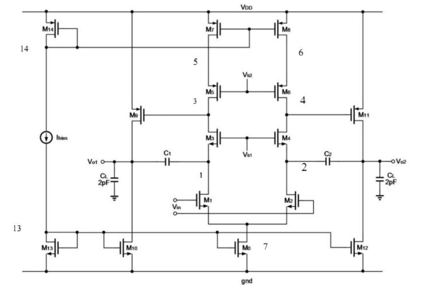
Circuit Sizing for Op. Amp.

• Geometric Programming formulation for CMOS Op. Amp.
• Min-max convex programming under Parametric variations (PVT)
• Ellipsoid Method

What is Affine Arithmetic?

• Represents a quantity x with an affine form (AAF): $$\hat{x}=x_0+x_1{ϵ}_1+\dots +x_n{ϵ}_n$$ where
  • noise symbols ${ϵ}_i\in [-1,1]$
  • central value $x_0\in \mathbb{R}$
  • partial deviations $x_i\in \mathbb{R}$
  • $n$ is not fixed - new noise symbols are generated during the computation process.
• IA -> AA : $[\mathrm{3..4}]\to 3.5+0.5{ϵ}_1$

Geometry of AA

• Affine forms that share noise symbols are dependent:
  • $\hat{x}=x_0+x_1{ϵ}_1+\dots +x_n{ϵ}_n$
  • $\hat{y}=y_0+y_1{ϵ}_1+\dots +y_m{ϵ}_m$
• The region containing (x, y) is:
  • $Z=\{(x,y):{ϵ}_i\in [-1,1]\}$
  • This region is a centrally symmetric convex polygon called "zonotope".

Affine Arithmetic

How to find ${\sup }_{q\in \mathbb{Q}}{f}_j(x,q)$ efficiently?

• ${\sup }_{q\in \mathbb{Q}}{f}_j(x,q)$ is in general difficult to obtain.
• Provided that variations are small or nearly linear, we propose using Affine Arithmetic (AA) to solve this problem.
• Features of AA:
  • Handle correlation of variations by sharing noise symbols.
  • Enabling technology: template and operator overloading features of C++.
  • A C++ package "YALAA" is publicly available.

Affine Arithmetic for Worst Case Analysis

• An uncertain quantity is represented in an affine form (AAF): $$\hat{a}=a_0+a_1{\epsilon }_1+a_2{\epsilon }_2+\cdots +a_k{\epsilon }_k=a_0+\sum _{i=1}^k{a}_i{\epsilon }_i,$$ where
  • ${\epsilon }_i\in [-1,1]$ is called noise symbol.
• Exact results for affine operations ($\hat{a}+\hat{b}$, $\hat{a}-\hat{b}$ and $\alpha \cdot \hat{a}$)
• Results of non-affine operations (such as $\hat{a}\cdot \hat{b}$, $\hat{a}/\hat{b}$, $\max (\hat{a},\hat{b}),\log (\hat{a})$) are approximated in an affine form.
• AA has been applied to a wide range of applications recently when process variations are considered.

Affine Arithmetic for Optimization

In our robust GP problem:

• First, represent every elements in $q$ in affine forms.
• For each ellipsoid iteration, $f(x_c,q)$ is obtained by approximating $f(x_c,\hat{q})$ in an affine form: $$\hat{f}=f_0+f_1{\epsilon }_1+f_2{\epsilon }_2+\cdots +f_k{\epsilon }_k.$$
• Then the maximum of $\hat{f}$ is determined by: $${\epsilon }_j=\{\begin{array}{ll}+1& \text{if}{f}_j>0\\ -1& \text{if}{f}_j<0\end{array}j=1,\cdots ,k.$$

Performance Specification

Open-Loop Gain (Example)

• Open-loop gain $A_v$ can be approximated as a monomial function:

  $$A_v=\frac{2C_{ox}}{({\lambda }_n+{\lambda }_p{)}^2}\sqrt{{\mu }_n{\mu }_p\frac{W_1{W}_6}{L_1{L}_6{I}_1{I}_6}}$$

  where $I_1$ and $I_6$ are monomial functions.

• Corresponding C++ code fragment:

  // Open Loop Gain
  monomial<aaf> OLG = 2*COX/square(LAMBDAN+LAMBDAP)*
       sqrt(KP*KN*W[1]/L[1]*W[6]/L[6]/I1/I6);
  

Results of Design Variables

Performances

Conclusions

• Our ellipsoid method is fast enough for practical analog circuit sizing (take < 1 sec. running on a 3GHz Intel CPU for our example).
• Our method is reliable, in the sense that the solution, once produced, always satisfies the specification requirement in the worst case.

Comments

• The marriage of AA (algebra) and Zonotope (geometry) has the potential to provide us with a powerful tool for algorithm design.
• AA does not solve all problems. E.g. Iterative method does not apply to AA because AA is not in the Banach space (the fixed-point theorem does not hold).
• AA * and + do not obey the laws of distribution (c.f. floating-point arithmetic)
• AA can only perform first-order approximations. In other words, it can only be applied to nearly linear variations.
• In practice, we still need to combine AA with other methods, such as statistical method or the (quasi-) Monte Carlo method.