Lecture 8: Phase Shifting Mask

@luk036

2022-11-26

🗺️ Overview

• Background
• What is Phase Shifting Mask?
• Phase Conflict Graph
• Phase Assignment Problem
  • Greedy Approach
  • Planar Graph Approach

class: middle, center

Background

Background

.pull-left[

• In the past, chips have continued to get smaller and smaller, and therefore consume less and less power.

• However, we are rapidly approaching the end of the road and optical lithography cannot take us to the next place we need to go.

] .pull-right[

]

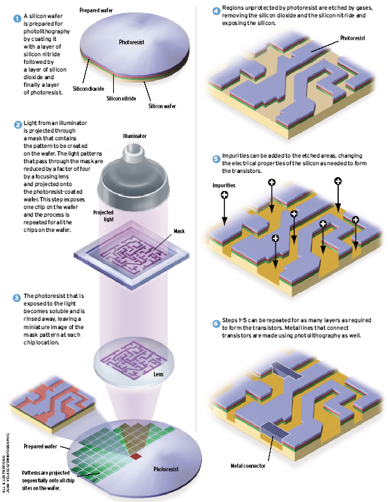
Process of Lithography

.pull-left[

1. Photo-resist coating (光阻涂层)

2. Illumination (光照)

3. Exposure (曝光)

4. Etching (蚀刻)

5. Impurities doping (杂质掺杂)

6. Metal connection

] .pull-right[

]

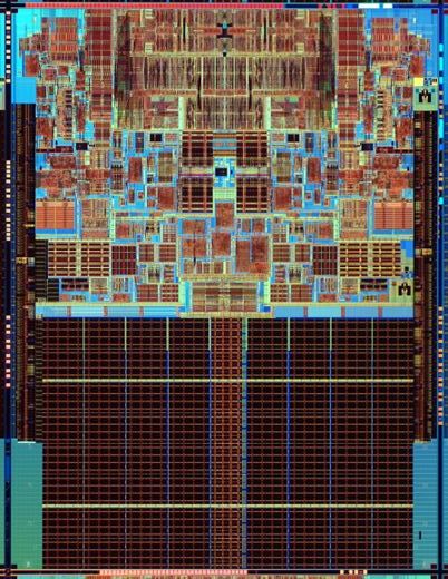
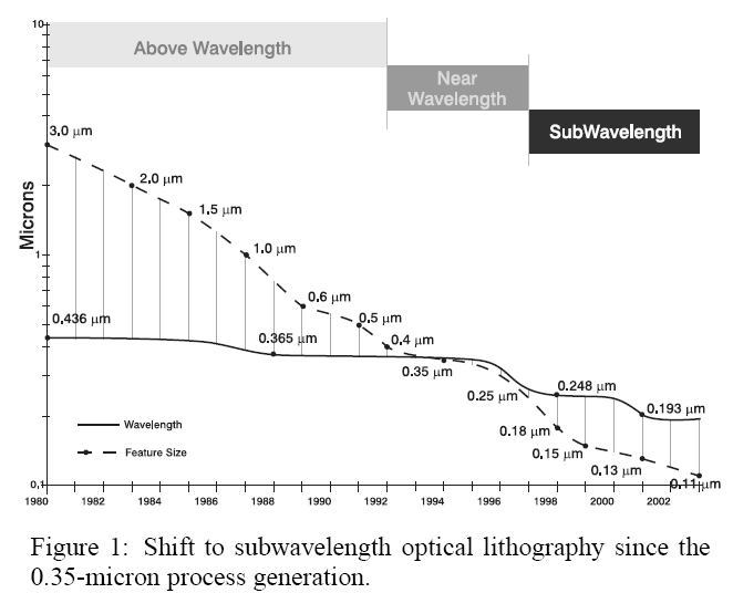
Sub-wavelength Lithography

.pull-left[

• Feature size is much smaller than the lithography wavelength
  • 45nm vs. 193nm

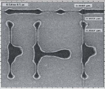
] .pull-right[

• What you see in the mask/layout is not what you get on the chip:
  • Features are distored
  • Yields are declined

]

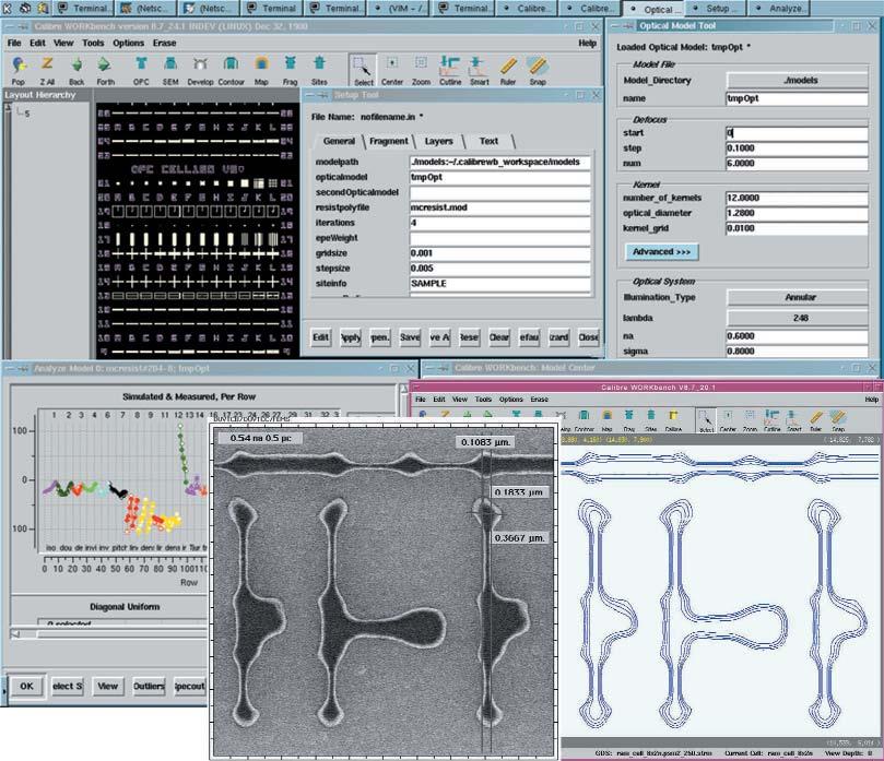
DFM Tool (Mentor Graphics)

OPC and PSM

.pull-left[

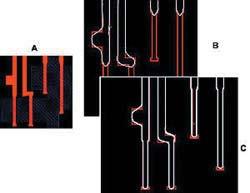
• Results of OPC on PSM:
  • A = original layout
  • B = uncorrected layout
  • C = after PSM and OPC

] .pull-right[

]

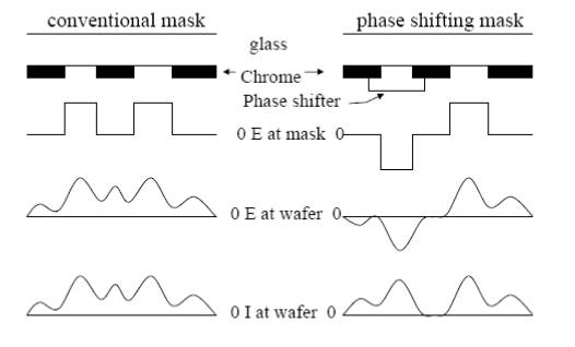
Phase Shifting Mask

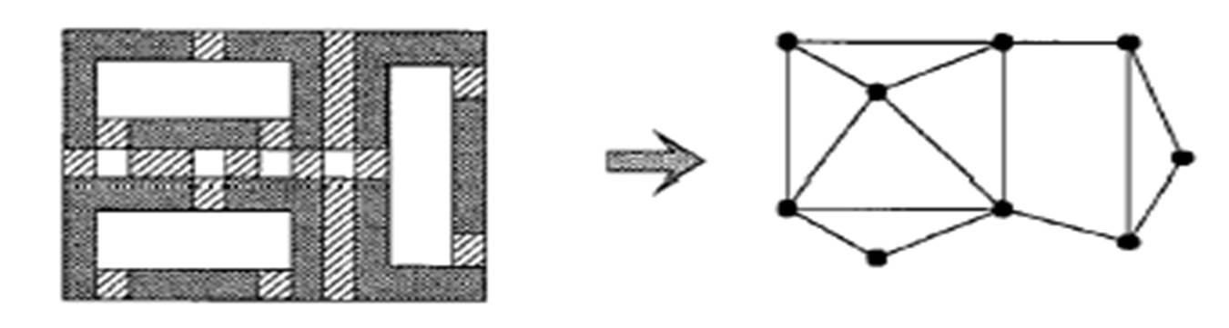
Phase Conflict Graph

• Edge between two features with separation of $\le b$ (dark field)
• Similar conflict graph for "bright field".
• Construction method: plane sweeping method + dynamic priority search tree

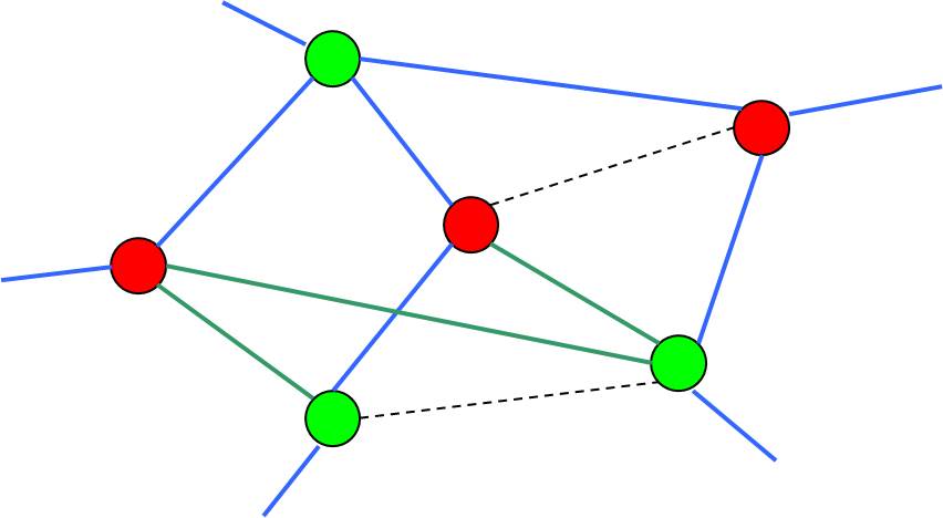
Phase Assignment Problem

.pull-left[

• Instance: Graph $G=(V,E)$
• Solution: A color assignment $c:V\to [\mathrm{1..}k]$ (here $k=2$)
• Goal: Minimize the weights of the monochromatic edges. (Question: How can we model the weights?)

] .pull-right[

]

Phase Assignment Problem

• In general, the problem is NP-hard.
• It is solvable in polynomial time for planar graphs with $k=2$, since the problem is equivalent to the T-join problem in the dual graph [Hadlock75].
• For planar graphs with $k=2$, the problem can be solved approximately in the ratio of two using the primal-dual method.

Overview of Greedy Algorithm

• Create a maximum weighted spanning tree (MST) of $G$ (can be found in LEDA package)
• Assign colors to the nodes of the MST.
• Reinsert edges that do not conflict.
• Time complexity: $O(N\log N)$
• Can be applied to non-planar graphs.

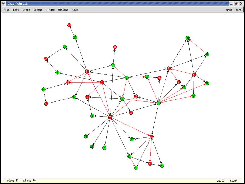
Greedy Algorithm

.pull-left[

• Step 1: Construct a maximum spanning tree $T$ of $G$ (using e.g. Kruskal's algorithm, which is available in the LEDA package).

] .pull-right[

]

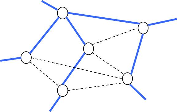
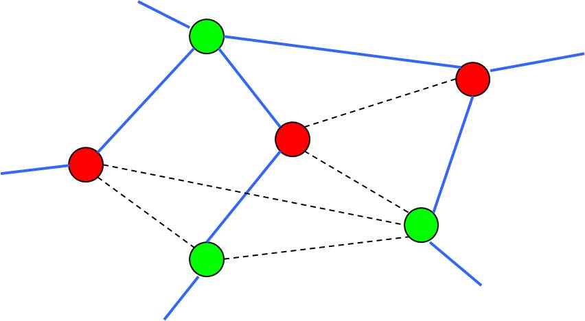
Greedy Algorithm (Cont'd)

.pull-left[

• Step 2: Assign colors to the nodes of $T$.

] .pull-right[

]

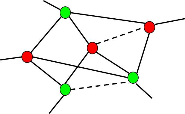
Greedy Algorithm (Cont'd)

.pull-left[

• Step 3: Reinsert edges that do not conflict.

] .pull-right[

]

Other Approaches

• Reformulate the problem as a MAX-CUT problem. Note that the MAX-CUT problem is approximatable within a factor of 1.1383 using the "semi-definite programming" relaxation technique [Goemans and Williamson 93].

• Planar graph approach: Convert $G$ to a planar graph by removing the minimal edges, and then apply the methods to the resulting planar graph.

  👉 Note: the optimal "planar sub-graph" problem is NP-hard.

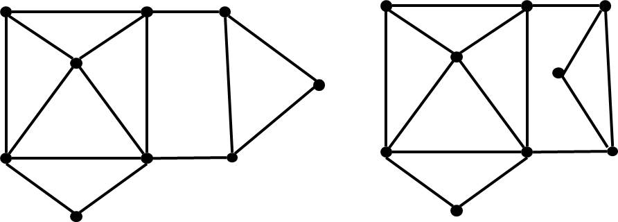
Overview of Planar Graph Approach (Hadlock's algorithm)

1. Approximate $G$ by a planar graph $G^{\prime }$
2. Decompose $G^{\prime }$ into its bi-connected components.
3. For each bi-connected component in $G^{\prime }$,
   1. construct a planar embedding
   2. construct a dual graph $G^{\ast }$
   3. construct a complete graph $C(V,E)$, where
      • $V$ is a set of odd-degree vertices in $G^{\ast }$
      • the weight of each edge is the shortest path of two vertices
   4. find the minimum perfect matching 💯👬🏻 solution. The matching edges are the conflict edges that have to be deleted.
4. Reinsert the non-conflicting edges from $G$.

Planar Graph Approach

.pull-left[

• Step 1: Approximate $G$ with a planar graph $G^{\prime }$
  • It is NP-hard.
  • The naive greedy algorithm takes $O(n^2)$ time.
  • Any good suggestion?

] .pull-right[

]

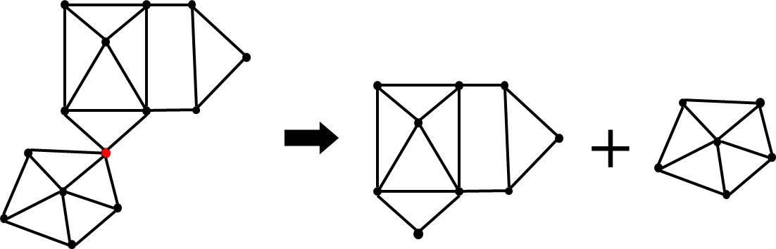
Planar Graph Approach

• Step 2: Decompose $G^{\prime }$ into its bi-connected components in linear time (available in the LEDA package).

  

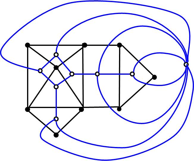
Planar Graph Approach

• Step 3: For each bi-connected component in $G^{\prime }$, construct a planar embedding in linear time (available in the LEDA package)

  

👉 Note: planar embedding may not be unique unless $G$ is tri-connected.

Planar Graph Approach

.pull-left[

• Step 4: For each bi-connected component, construct its dual graph $G^{\ast }$ in linear time.

] .pull-right[

]

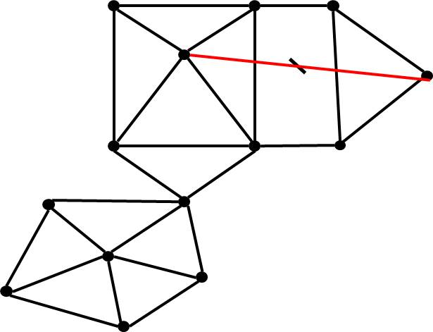
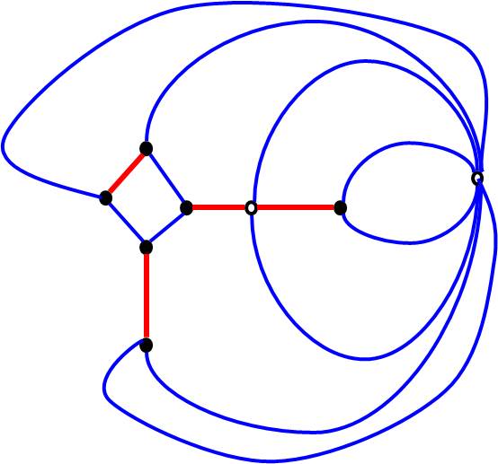
Planar Graph Approach

.pull-left[

• Step 5: Find the minimum weight perfect matching 💯👬🏻 of $G^{\ast }$.

  • Polynomial time solvable.
  • Can be formulated as a network flow problem.

  👉 Note: complete graph vs. Voronoi graph

] .pull-right[

]

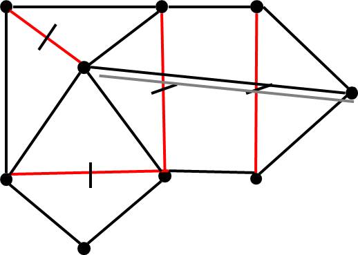
Planar Graph Approach

.pull-left[

• Step 6: reinsert the non-conflicting edges in $G$.

👉 Note: practically we keep track of conflicting edges.

] .pull-right[

]