When "Convex Optimization" Meets "Network Flow"

📖 Introduction

Overview

• Network flow problems can be solved efficiently and have a wide range of applications.

• Unfortunately, some problems may have other additional constraints that make them impossible to solve with current network flow techniques.

• In addition, in some problems, the objective function is quasi-convex rather than convex.

• In this lecture, we will investigate some problems that can still be solved by network flow techniques with the help of convex optimization.

Parametric Potential Problems

Parametric potential problems

Consider:

$$\begin{array}{ll}\text{maximize}& g(\beta ),\\ \text{subject to}& y\le d(\beta ),\\ & Au=y,\end{array}$$

where $g(\beta )$ and $d(\beta )$ are concave.

Note: the parametric flow problems can be defined in a similar way.

Network flow says:

• For fixed $\beta$, the problem is feasible precisely when there exists no negative cycle

• Negative cycle detection can be done efficiently using the Bellman-Ford-like methods

• If a negative cycle $C$ is found, then ${\sum }_{(i,j)\in C}{d}_{ij}(\beta )<0$

Convex Optimization says:

• If both sub-gradients of $g(\beta )$ and $d(\beta )$ are known, then the bisection method can be used for solving the problem efficiently.

• Also, for multi-parameter problems, the ellipsoid method can be used.

Quasi-convex Minimization

Consider: $$\begin{array}{ll}\text{maximize}& f(\beta ),\\ \text{subject to}& y\le d(\beta ),\\ & Au=y,\end{array}$$

where $f(\beta )$ is quasi-convex and $d(\beta )$ are concave.

Example of Quasi-Convex Functions

• $\sqrt{|y|}$ is quasi-convex on $\mathbb{R}$

• $\log (y)$ is quasi-linear on ${\mathbb{R}}_{++}$

• $f(x,y)=xy$ is quasi-concave on ${\mathbb{R}}_{++}^2$

• Linear-fractional function:

  • $f(x)$ = $(a^{\mathsf{T}}x+b)/(c^{\mathsf{T}}x+d)$

  • dom $f$ = $\{x|c^{\mathsf{T}}x+d>0\}$

• Distance ratio function:

  • $f(x)$ = $\Vert x-a{\Vert }_2/\Vert x-b{\Vert }_2$

  • dom $f$ = $\{x|\Vert x-a{\Vert }_2\le \Vert x-b{\Vert }_2\}$

Convex Optimization says:

If $f$ is quasi-convex, there exists a family of functions ${\varphi }_t$ such that:

• ${\varphi }_t(\beta )$ is convex w.r.t. $\beta$ for fixed $t$

• ${\varphi }_t(\beta )$ is non-increasing w.r.t. $t$ for fixed $\beta$

• $t$-sublevel set of $f$ is $0$-sublevel set of ${\varphi }_t$, i.e., $f(\beta )\le t$ iff ${\varphi }_t(\beta )\le 0$

For example:

• $f(\beta )=p(\beta )/q(\beta )$ with $p$ convex, $q$ concave $p(\beta )\ge 0$, $q(\beta )>0$ on dom $f$,

• can take ${\varphi }_t(\beta )$ = $p(\beta )-t\cdot q(\beta )$

Convex Optimization says:

Consider a convex feasibility problem: $$\begin{array}{ll}\text{find}& f(\beta ),\\ \text{s. t.}& {\varphi }_t(\beta )\le 0,\\ & y\le d(\beta ),Au=y,\end{array}$$

• If feasible, we conclude that $t\ge p^{\ast }$;

• If infeasible, $t<p^{\ast }$.

Binary search on $t$ can be used for obtaining $p^{\ast }$.

Quasi-convex Network Problem

• Again, the feasibility problem ([eq:quasi]) can be solved efficiently by the bisection method or the ellipsoid method, together with the negatie cycle detection technique.

• Any EDA's applications ???

Monotonic Minimization

• Consider the following problem: $$\begin{array}{ll}\text{minimize}& {\max }_{ij}{f}_{ij}(y_{ij}),\\ \text{subject to}& Au=y,\end{array}$$

  where $f_{ij}(y_{ij})$ is non-decreasing.

• The problem can be recast as:

  $$\begin{array}{ll}\text{maximize}& \beta ,\\ \text{subject to}& y\le f^{-1}(\beta ),\\ & Au=y,\end{array}$$

  where $f^{-1}(\beta )$ is non-deceasing w.r.t. $\beta$.

E.g. Yield-driven Optimization

• Consider the following problem:

  $$\begin{array}{ll}\text{maximize}& {\min }_{ij}\mathrm{Pr}(y_{ij}\le {\tilde{d}}_{ij})\\ \text{subject to}& Au=y,\end{array}$$

  where ${\tilde{d}}_{ij}$ is a random variables.

• Equivalent to the problem:

  $$\begin{array}{ll}\text{maximize}& \beta ,\\ \text{subject to}& \beta \le \mathrm{Pr}(y_{ij}\le {\tilde{d}}_{ij}),\\ & Au=y,\end{array}$$

  where $f_{ij}^{-1}(\beta )$ is non-deceasing w.r.t. $\beta$.

E.g. Yield-driven Optimization (II)

• Let $F(x)$ is the cdf of $\tilde{d}$.

• Then: $$\begin{array}{lll}& & \beta \le \mathrm{Pr}(y_{ij}\le {\tilde{d}}_{ij})\le t\\ & \Rightarrow & \beta \le 1-F_{ij}(y_{ij})\\ & \Rightarrow & y_{ij}\le F_{ij}^{-1}(1-\beta )\end{array}$$

• The problem becomes:

  $$\begin{array}{ll}\text{maximize}& \beta ,\\ \text{subject to}& y_{ij}\le F_{ij}^{-1}(1-\beta ),\\ & Au=y,\end{array}$$

Network flow says

• Monotonic problem can be solved efficiently using cycle-cancelling methods such as Howard's algorithm.

Min-cost flow problems

Min-Cost Flow Problem (linear)

Consider:

$$\begin{array}{ll}\text{min}& d^{\mathsf{T}}x+p\\ \text{s. t.}& c^{-}\le x\le c^{+},\\ & A^{\mathsf{T}}x=b,b(V)=0\end{array}$$

• some $c^{+}$ could be $+\infty$ some $c^{-}$ could be $-\infty$.
• $A^{\mathsf{T}}$ is the incidence matrix of a network $G$.

Conventional Algorithms

• Augmented-path based:
  • Start with an infeasible solution
  • Inject minimal flow into the augmented path while maintaining infeasibility in each iteration
  • Stop when there is no flow to inject into the path.
• Cycle cancelling based:
  • Start with a feasible solution $x_0$
  • find a better sol'n $x_1=x_0+\alpha △x$, where $\alpha$ is positive and $△x$ is a negative cycle indicator.

General Descent Method

1. Input: a starting $x\in$ dom $f$
2. Output: $x^{\ast }$
3. repeat
   1. Determine a descent direction $p$.
   2. Line search. Choose a step size $\alpha >0$.
   3. Update. $x:=x+\alpha p$
4. until a stopping criterion is satisfied.

Some Common Descent Directions

• For convex problems, the search direction must satisfy $\nabla f(x{)}^{\mathsf{T}}p<0$.
• Gradient descent:
  • $p=-\nabla f(x{)}^{\mathsf{T}}$
• Steepest descent:
  • $△x^{nsd}=\mathrm{argmin}\{\nabla f(x{)}^{\mathsf{T}}v\mid \Vert v\Vert =1\}$.
  • $△x^{sd}$ = $\Vert \nabla f(x)\Vert △x^{nsd}$ (un-normalized)
• Newton's method:
  • $p=-{\nabla }^{2}f(x{)}^{-1}\nabla f(x)$

Network flow says (II)

• Here, there is a better way to choose $p$!
• Let $x:=x+\alpha p$, then we have: $$\begin{array}{lll}\text{min}& d^{\mathsf{T}}{x}_0+\alpha d^{\mathsf{T}}p& \Rightarrow d^{\mathsf{T}}<0\\ \text{s. t.}& -x_0\le \alpha p\le c-x_0& \Rightarrow \text{residual graph}\\ & A^{\mathsf{T}}p=0& \Rightarrow p\text{ is a cycle!}\end{array}$$
• In other words, choose $p$ to be a negative cycle with cost $d$!
  • Simple negative cycle, or
  • Minimum mean cycle

Network flow says (III)

• Step size is limited by the capacity constraints:
  • ${\alpha }_1={\min }_{ij}\{c^{+}-x_0\}$, for $△x_{ij}>0$
  • ${\alpha }_2={\min }_{ij}\{x_0-c^{-}\}$, for $△x_{ij}<0$
  • ${\alpha }_{\mathrm{lin}}$ = min$\{{\alpha }_1,{\alpha }_2\}$
• If ${\alpha }_{\mathrm{lin}}=+\infty$, the problem is unbounded.

Network flow says (IV)

• An initial feasible solution can be obtained by a similar construction of the residual graph and cost vector.
• The LEMON package implements this cycle cancelling algorithm.

Min-Cost Flow Convex Problem

• Problem Formulation: $$\begin{array}{ll}\text{min}& f(x)\\ \text{s. t.}& 0\le x\le c,\\ & A^{\mathsf{T}}x=b,b(V)=0\end{array}$$

Common Types of Line Search

• Exact line search:
  • $t={\mathrm{argmin}}_{t>0}f(x+t△x)$
• Backtracking line search (with parameters $\alpha \in (0,1/2),\beta \in (0,1)$)
  • starting from $t=1$, repeat $t:=\beta t$ until $$f(x+t△x)<f(x)+\alpha t\nabla f(x{)}^{\mathsf{T}}△x$$
  • graphical interpretation: backtrack until $t\le t_0$

Network flow says (V)

• The step size is further limited by the following:
  • ${\alpha }_{\mathrm{cvx}}=\min \{{\alpha }_{\mathrm{lin}},t\}$
• In each iteration, choose $△x$ as a negative cycle of $G_x$, with cost $\nabla f(x)$ such that $\nabla f(x{)}^{\mathsf{T}}△x<0$

Quasi-convex Minimization (new)

• Problem Formulation: $$\begin{array}{ll}\text{min}& f(x)\\ \text{s. t.}& 0\le x\le c,\\ & A^{\mathsf{T}}x=b,b(V)=0\end{array}$$

• The problem can be recast as: $$\begin{array}{ll}\text{min}& t\\ \text{s. t.}& f(x)\le t,\\ & 0\le x\le c,\\ & A^{\mathsf{T}}x=b,b(V)=0\end{array}$$

Convex Optimization says (II)

• Consider a convex feasibility problem: $$\begin{array}{ll}\text{find}& x\\ \text{s. t.}& {\varphi }_t(x)\le 0,\\ & 0\le x\le c,\\ & A^{\mathsf{T}}x=b,b(V)=0\end{array}$$
  • If feasible, we conclude that $t\ge p^{\ast }$;
  • If infeasible, $t<p^{\ast }$.
• Binary search on $t$ can be used for obtaining $p^{\ast }$.

Network flow says (VI)

• Choose $△x$ as a negative cycle of $G_x$ with cost $\nabla {\varphi }_t(x)$
• If no negative cycle is found, and ${\varphi }_t(x)>0$, we conclude that the problem is infeasible.
• Iterate until $x$ becomes feasible, i.e. ${\varphi }_t(x)\le 0$.

E.g. Linear-Fractional Cost

• Problem Formulation: $$\begin{array}{ll}\text{min}& (e^{\mathsf{T}}x+f)/(g^{\mathsf{T}}x+h)\\ \text{s. t.}& 0\le x\le c,\\ & A^{\mathsf{T}}x=b,b(V)=0\end{array}$$

• The problem can be recast as: $$\begin{array}{ll}\text{min}& t\\ \text{s. t.}& (e^{\mathsf{T}}x+f)-t(g^{\mathsf{T}}x+h)\le 0\\ & 0\le x\le c,\\ & A^{\mathsf{T}}x=b,b(V)=0\end{array}$$

Convex Optimization says (III)

• Consider a convex feasibility problem: $$\begin{array}{ll}\text{find}& x\\ \text{s. t.}& (e-t\cdot g{)}^{\mathsf{T}}x+(f-t\cdot h)\le 0,\\ & 0\le x\le c,\\ & A^{\mathsf{T}}x=b,b(V)=0\end{array}$$
  • If feasible, we conclude that $t\ge p^{\ast }$;
  • If infeasible, $t<p^{\ast }$.
• Binary search on $t$ can be used for obtaining $p^{\ast }$.

Network flow says (VII)

• Choose $△x$ to be a negative cycle of $G_x$ with cost $(e-t\cdot g)$, i.e. $(e-t\cdot g{)}^{\mathsf{T}}△x<0$
• If no negative cycle is found, and $(e-t\cdot g{)}^{\mathsf{T}}{x}_0+(f-t\cdot h)>0$, we conclude that the problem is infeasible.
• Iterate until $(e-t\cdot g{)}^{\mathsf{T}}{x}_0+(f-t\cdot h)\le 0$.

E.g. Statistical Optimization

• Consider the quasi-convex problem:

  $$\begin{array}{ll}\text{min}& \mathrm{Pr}({\mathbf{d}}^{\mathsf{T}}x>\alpha )\\ \text{s. t.}& 0\le x\le c,\\ & A^{\mathsf{T}}x=b,b(V)=0\end{array}$$

  • $\mathbf{d}$ is random vector with mean $d$ and covariance $\Sigma$.
  • Hence, ${\mathbf{d}}^{\mathsf{T}}x$ is a random variable with mean $d^{\mathsf{T}}x$ and variance $x^{\mathsf{T}}\Sigma x$.

📈 Statistical Optimization

• The problem can be recast as: $$\begin{array}{ll}\text{min}& t\\ \text{s. t.}& \mathrm{Pr}({\mathbf{d}}^{\mathsf{T}}x>\alpha )\le t\\ & 0\le x\le c,\\ & A^{\mathsf{T}}x=b,b(V)=0\end{array}$$

👉 Note: $$\begin{array}{lll}& & \mathrm{Pr}({\mathbf{d}}^{\mathsf{T}}x>\alpha )\le t\\ & \Rightarrow & d^{\mathsf{T}}x+F^{-1}(1-t)\Vert {\Sigma }^{1/2}x{\Vert }_2\le \alpha \end{array}$$ (convex quadratic constraint w.r.t $x$)

Recall...

Recall that the gradient of $d^{\mathsf{T}}x+F^{-1}(1-t)\Vert {\Sigma }^{1/2}x{\Vert }_2$ is $d+F^{-1}(1-t)(\Vert {\Sigma }^{1/2}x{\Vert }_2{)}^{-1}\Sigma x$.

Problem w/ additional Constraints (new)

• Problem Formulation: $$\begin{array}{ll}\text{min}& f(x)\\ \text{s. t.}& 0\le x\le c,\\ & A^{\mathsf{T}}x=b,b(V)=0\\ & s^{\mathsf{T}}x\le \gamma \end{array}$$

E.g. Yield-driven Delay Padding

• Consider the following problem: $$\begin{array}{ll}\text{maximize}& \gamma \beta -c^{\mathsf{T}}p,\\ \text{subject to}& \beta \le \mathrm{Pr}(y_{ij}\le {\mathbf{d}}_{ij}+p_{ij}),\\ & Au=y,p\ge 0\end{array}$$

  • $p$: delay padding
  • $\gamma$: weight (determined by a trade-off curve of yield and buffer cost)
  • ${\mathbf{d}}_{ij}$: Gaussian random variable with mean $d_{ij}$ and variance $s_{ij}$.

E.g. Yield-driven Delay Padding (II)

• The problem is equivalent to: $$\begin{array}{ll}\text{max}& \gamma \beta -c^{\mathsf{T}}p,\\ \text{s.t.}& y\le d-\beta s+p,\\ & Au=y,p\ge 0\end{array}$$

• or its dual: $$\begin{array}{ll}\text{min}& d^{\mathsf{T}}x\\ \text{s.t.}& 0\le x\le c,\\ & A^{\mathsf{T}}x=b,b(V)=0\\ & s^{\mathsf{T}}x\le \gamma \end{array}$$

Recall ...

• Yield drive CSS: $$\begin{array}{ll}\text{max}& \beta ,\\ \text{s.t.}& y\le d-\beta s,\\ & Au=y,\end{array}$$

• Delay padding $$\begin{array}{ll}\text{max}& -c^{\mathsf{T}}p,\\ \text{s.t.}& y\le d+p,\\ & Au=y,p\ge 0\end{array}$$

Considering Barrier Method

• Approximation via logarithmic barrier:

  $$\begin{array}{ll}\text{min}& f(x)+(1/t)\varphi (x)\\ \text{s.t.}& 0\le x\le c,\\ & A^{\mathsf{T}}x=b,b(V)=0\end{array}$$

  • where $\varphi (x)=-\log (\gamma -s^{\mathsf{T}}x)$
  • Approximation improves as $t\to \infty$
  • Here, $\nabla \varphi (x)=s/(\gamma -s^{\mathsf{T}}x)$

Barrier Method

• Input: a feasible $x$, $t:=t^{(0)}$, $\mu >1$, tolerance $\epsilon >0$
• Output: $x^{\ast }$
• repeat
  1. Centering step. Compute $x^{\ast }(t)$ by minimizing $tf+\varphi$
  2. Update $x:=x^{\ast }(t)$.
  3. Increase $t$. $t:=\mu t$
• until $1/t<\epsilon$.

👉 Note: Centering is usually done by Newton's method in general.

Network flow says (VIII)

In the centering step, instead of using the Newton descent direction, we can replace it with a negative cycle on the residual graph.

Useful Skew Design Flow

Useful Skew Design: Why vs. Why Not {#sec:first}

Why not

Some common challenges when implementing useful skew design include:

• need more engineer training
• difficulty in building a balanced clock-tree
• uncertainty in how to handle process variation and multi-corner multi-mode issues ..., etc.

Why

If these challenges are overcome and useful skew design is implemented correctly,

• it can lead to less time spent on timing issues
• get better chip performance or yield

Clock Arrival Time vs. Clock Skew

• Clock signal runs periodically.

• Thus, absolute clock arrival time $u_i$ is not so important.

• Instead, the skew $y_{ij}=u_i-u_j$ is more important in this scenario.

Useful Skew Design vs. Zero-Skew Design

• "Critical cycle" instead of "critical path".
• "Negative cycle" instead of "negative slack".
• If there is a negative cycle, it means that there is no positive slack solution no matter how to schedule.
• Others are pretty much the same.
• Same design principle:
  • Always tackle the most critical one first!

Linear Programming vs. Network Flow Formulation

• Linear programming formulation
  • can handle more complex constraints
• Network flow formulation
  • usually more efficient
  • return the most critical cycle as a bonus
  • can handle quantized buffer delay (???)
• Anyway, timing analysis is much more time-consuming than the optimization solving.

Target Skew vs. Actual Skew

Don't mess up these two concepts:

• Target skew:
  • the skew we want to achieve in the scheduling stage.
  • Usually deterministic (we schedule a meeting at 10:00, rather than 10:00 $\pm$ 34 minutes, right?)
• Actual skew
  • the skew that the clock tree actually generates.
  • Can be formulated as a random variable.

A Simple Case

To warm up, let us start with a simple case:

• Assume equal path delay variations.
• Single-corner.
• Before a clock tree is built.
• No adjustable delay buffer (ADB).

Network

Definition (Network)

A network is a collection of finite-dimensional vector spaces of nodes and edges/arcs:

• $V=\{v_1,v_2,\cdots ,v_N\}$, where $|V|=N$
• $E=\{e_1,e_2,e_3,\cdots ,e_M\}$, where $|E|=M$

which satisfies 2 requirements:

1. The boundary of each edge is comprised of the union of nodes
2. The intersection of any edges is either empty or a boundary node of both edges.

Example

\begin{figure}[hp]
\centering
\input{lec07.files/network.tikz}
\caption{A network}%
\label{fig:network}
\end{figure}

Orientation

Definition (Orientation)

An orientation of an edge is an ordering of its boundary node $(s,t)$, where

• $s$ is called a source/initial node
• $t$ is called a target/terminal node

Definition (Coherent)

Two orientations to be the same is called coherent

Node-edge Incidence Matrix

Definition (Incidence Matrix)

A $N\times M$ matrix $A^{\mathsf{T}}$ is a node-edge incidence matrix with entries: $$A(i,j)=\{\begin{array}{ll}+1& \text{if ei is coherent with vj},\\ -1& \text{if ei is not coherent with vj},\\ 0& \text{otherwise.}\end{array}$$

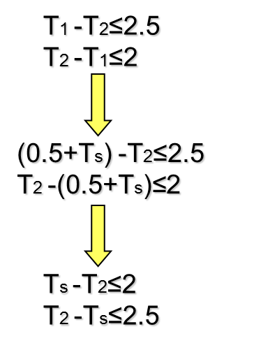
Timing Constraint

• Setup time constraint $$y_{\text{skew}}(i,f)\le T_{\text{CP}}-D_{if}-T_{\text{setup}}=u_{if}$$ While this constraint destroyed, cycle time violation (zero clocking) occurs.
• Hold time constraint $$y_{\text{skew}}(i,f)\ge T_{\text{hold}}-d_{if}=l_{if}$$ While this constraint destroyed, race condition (double clocking) occurs.

Timing Constraint Graph

• Create a graph (network) by
  • replacing the hold time constraint with an h-edge with cost $-(T_{\text{hold}}-d_{ij})$ from ${\text{FF}}_i$ to ${\text{FF}}_j$, and
  • replacing the setup time constraint with an s-edge with cost $T_{\text{CP}}-D_{ij}-T_{\text{setup}}$ from ${\text{FF}}_j$ to ${\text{FF}}_i$.
• Two sets of constraints stemming from clock skew definition:
  • The sum of skews for paths having the same starting and ending flip-flop to be the same;
  • The sum of clock skews of all cycles to be zero

Timing Constraint Graph (TCG)

\begin{figure}[h!]
\centering
\input{lec05.files/tcgraph.tikz}
\end{figure}

First Thing First

Meet all timing constraints

• Find $y$ in $\{y\in {\mathbb{R}}^n\mid y\le d,Au=y\}$
• How to solve:
  1. Find a negative cycle, fix it.
  2. Iterate until no negative cycle is found.
• Bellman-Ford-like algorithm (and its variants are publicly available):
  • Strongly suggest "Lazy Evaluation":
    • Don't do full timing analysis on the whole timing graph at the beginning!
    • Instead, perform timing analysis only when the algorithm needs.
  • Stop immediately whenever a negative cycle is detected.

Delay Padding (DP)

• Delay padding is a technique that fixes the timing issue by intentionally solely "increasing" delays.
• Usually formulated as:
  • Find $p,y$ in $\{p,y\in {\mathbb{R}}^n\mid y\le d+p,Au=y,p\ge 0\}$
• If the objective is to minimize the sum of $p$, then the problem is the dual of the standard min-cost flow problem, which can be solved efficiently by the network simplex algorithm (publicly available).
• Beautiful right?

Delay Padding (II)

• No, the above formulation is impractical.
• In modern design, "inserting" a delay may mean swapping a faster cell with a slower cell from the cell library. Thus, no need to minimize the sum of $p$.
• More importantly, it may not be possible to find a position to insert delay for some delay paths.
• Some papers consider only allowing insert delays to the max-delay path only. Some papers consider only allowing insert delays to both the max- and min-delay paths together only. None of them are perfect.

Delay Padding (III)

• My suggestion. Instead of calculating the necessary $p^{\prime }s$ and then look for the suitable position to insert, it is easier (and more flexible) to determine the position first and then calculate the suitable values.
• It can be achieved by modifying the timing graph and solve a feasibility problem. Easy enough!
• Quantized delay can be handled too (???).

Four possible ways to insert delay

\begin{figure}[htpb]
\centering
\subfigure[No delay can be inserted]{
\input{lec07.files/no_delay.tikz}
}
\subfigure[$p_s$, $p_h$ independently]{
\input{lec07.files/independent.tikz}
}
\subfigure[$p_s = p_h$]{
\input{lec07.files/same_delay.tikz}
}
\subfigure[$p_s \geq p_h$]{
\input{lec07.files/setup_greater.tikz}
}
\caption{}
\end{figure}

Delay Padding (cont'd)

• If there exists a negative cycle in the modified timing graph, it implies that the timing problem cannot be fixed by simply the delay padding technique.
  • Then, try decrease $D_{ij}$, or increase $T_{\text{CP}}$
• Be aware of the min-delay path is still the min-delay path after a certain amount of delay is inserted (how???).

Variation Issue

Yield-driven Clock Skew Scheduling

• Assume all timing issues are fixed.
• Now, how to schedule the arrival times to maximize yield?
• According to the critical-first principle, we seek for the most critical cycle first.
• The problem can be formulated as:
  • $\max \{\beta \in \mathbb{R}\mid y\le d-\beta ,Au=y\}$.
• It is equivalent to the minimum mean cycle problem, which can be solved efficiently by for example Howard's algorithm (publicly available).

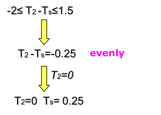
Minimum Balancing Algorithm

• Then we evenly distribute the slack on this cycle.
• To continue the next most critical cycle, we contract the first one into a "super vertex" and repeat the process.
• The process stops when the timing graph remains only a single vertex.
• The overall method is known as minimum balancing (MB) algorithm in the literature.

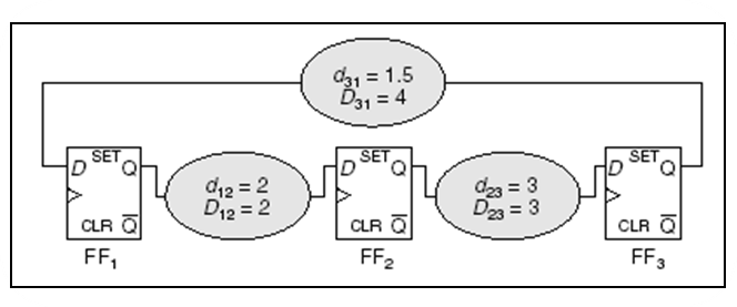
Example: Most timing-critical cycle

The most vulnerable timing constraint

\input{lec05.files/tcgraph2.tikz}

Example: Distribute the slack

• Distribute the slack evenly along the most timing-critical cycle.

\input{lec05.files/tcgraph3.tikz}

Example: Distribute the slack (cont'd)

• To determine the optimal slacks and skews for the rest of the graph, we replace the critical cycle with a super vertex.

\input{lec05.files/tcgraph4.tikz}
\input{lec05.files/tcgraph5.tikz}

Repeat the process iteratively

\input{lec05.files/tcgraph6.tikz}

Repeat the process iteratively (II)

\input{lec05.files/tcgraph7.tikz}

Final result

• Skew${}_{12}$ = 0.75

• Skew${}_{23}$ = -0.25

• Skew${}_{31}$ = -0.5

• Slack${}_{12}$ = 1.75

• Slack${}_{23}$ = 1.75

• Slack${}_{31}$ = 1

  where Slack${}_{ij}$ = CP - D${}_{ij}$ - T${}_{\text{setup}}$ - Skew${}_{ij}$

\begin{tikzpicture}
\def \radius {2cm}

\node[draw, circle, fill=cyan!20] at ({30}:\radius) (n1) {0.25};
\node[draw, circle, fill=cyan!20] at ({150}:\radius) (n2) {0.75};
\node[draw, circle, fill=cyan!20] at ({270}:\radius) (n3) {0};

\path[->, >=latex] (n2) edge [bend left=45] node[above]{0.5} (n1);
\path[->, >=latex] (n3) edge [bend left=45] node[left]{2.5} (n2);
\path[->, >=latex] (n1) edge [bend left=45] node[right]{1.5} (n3);

\path[dashed, ->, >=latex] (n1) edge [bend left=15] node[above]{1.5} (n2);
\path[dashed, ->, >=latex] (n2) edge [bend left=15] node[left]{2} (n3);
\path[dashed, ->, >=latex] (n3) edge [bend left=15] node[right]{3} (n1);

\end{tikzpicture}

What the MB algorithm really give us?

• The MB algorithm not only give us the scheduling solution, but also a tree-topology that represents the order of "criticality"!

\begin{figure}
\centering
\input{lec05.files/hierachy.tikz}
\end{figure}

Clock-tree Synthesis and Placement

• I strongly suggest that the topology of the clock-tree precisely follows the order of "criticality"!
  • since the lower branch of clock-tree has smaller skew variation.
• I also suggest that the placer should follow the topology of the clock-tree:
  • Physically place the registers of the same branch together.
  • The locality implies stronger correlation of variations and implies even smaller skew variation due to the cancellation effect.
  • Note that the current SSTA does not provide the correlation information, so this is the best you can do!

Second Example: Yield-driven Clock Skew Scheduling

• Now assume that SSTA (or STA+OCV, POCV, AOCV) is performed.
• Let ($\bar{d}$, $s$) be the (mean, variance) of $\mathbf{d}$
• The most critical cycle can be obtained by solving:
  • $\max \{\beta \in \mathbb{R}\mid y\le \bar{d}-\beta s,Au=y\}$
• It is equivalent to the minimum cost-to-time ratio cycle problem, which can be solved efficiently by for example Howard's algorithm (publicly available).
• Gaussian distribution is assumed. For arbitrary distribution, see my DAC'08 paper.

What About the Correlation?

• In the above formulation, we minimum the maximum possibility of timing violation of each individual timing constraint. So only individual delay distribution is needed.
• Yes, the objective function is not the true timing-yield. But it is reasonable, easy to solve, and is the best you can do so far.

Multi-Corner Issue

Meet all timing constraints in Multi-Corner

• Assume no Adjustable Delay Buffer (ADB)
• Find $y$ in $\{y\in {\mathbb{R}}^n\mid y\le d^{(k)},Au=y,\forall k\in [\mathrm{1..}K]\}$
• Equivalent to finding $y$ in $\{y\in {\mathbb{R}}^n\mid y\le {\min }_k\{d^{(k)}\},Au=y\}$
• Feasibility problem
• How to solve:
  1. Find a negative cycle, fix it.
  2. Iterate until no negative cycle is found.
• Better avoid fixing the timing issue corner-by-corner. Inducing ping-pong effect.

Delay padding (DP) in Multi-Corner

• The problem CANNOT be formulated as a network flow problem. But still you can solve it by a linear programming formulation.
• Or, decompose the problem into sub-problems for each corner.
• Again use the modified timing graph technique.
• Then, $y$'s are shared variables of sub-problems.
• If we solve each sub-problem individually, the solution will not agree with each other. Induce ping-pong effect.
• Need something to drive the agreement.

Delay Padding (DP) in Multi-Corner (cont'd)

• Follow the idea of dual decomposition: If a solution is above the average. then introduce a punishment cost. If a solution is below the average, then introduce a rewarding cost.
• Then, each subproblem is a min-cost potential problem, which can be solved efficiently.
• If some subproblems do not have feasible solutions, it implies that the problem cannot be fixed by simply delay padding.
• The process repeats until all solutions converge. If not, it implies that the problem cannot be fixed by simply delay padding.

Yield-driven Clock Skew Scheduling

• $\max \{\beta \in \mathbb{R}\mid y\le d^{(k)}-\beta s,Au=y,\forall k\in [\mathrm{1..}K]\}$
• More or less the same as in Single Corner.

Clock-Tree Issue

Clock Tree Synthesis (CTS)

• Construct merging location
  • DME algorithm, Elmore delay, buffer insertion
• Some research on bounded-skew DME algorithm. But the algorithm is too complicated in my opinion.
• If the previous stage is over-optimized, the clock tree is hard to implement. If it happens, some budgeting techniques should be invoked (engineering issue)
• After a clock tree is constructed, more detailed timing (rather than Elmore delay) can be obtained via timing analysis.

Co-optimization Issue

• After a clock tree is built, we have a clearer picture.
• Should I perform the re-scheduling? And how?
• Some papers suggest adding a factor to the timing constraint, say: $$1.2u_i-0.8u_j\le w_{ij}$$.
• Then the formulation is not a kind of network-flow, but may still be solvable by linear programming.
• Need to investigate more deeply.

Adjustable Delay Buffer Issue

Adjustable delay buffers in Multi-Mode

• Assume adjustable delay buffers are added solely to the clock tree
• Hence, each mode can have a different set of arrival times.
• Easier for clock skew scheduling, harder for clock-tree synthesis.

Meet timing constraint in Multi-Mode:

• find $y^{(m)}$ in $\{y^{(m)}\in {\mathbb{R}}^n\mid y^{(m)}\le d^{(m)},A{u}^{(m)}=y^{(m)},\forall m\in [\mathrm{1..}M]\}$
• Can be done in parallel.
• find a negative cycle, fix it (do not need to know all $d_i^{(m)}$ at the beginning) for every mode in parallel.

Delay Padding (DP) in Multi-mode

• Again use a modified timing graph technique.
• NOT a network flow problem. Use LP, or
• Dual decomposition -> min-cost potential problem for each mode
  • Only $p$'s are shared variables.
  • Initial feasible solution obtained by the single-mode method
    • A negative cycle => problem cannot be fixed by DP
• Not converge => problem cannot be fixed by DP
  • Try decrease $D_{ij}$, or increase $T_{\text{CP}}$

Yield-driven Clock Skew Scheduling

• $\max \{\beta \in \mathbb{R}\mid y^{(m)}\le d^{(m)}-\beta s,A{u}^{(m)}=y^{(m)},\forall m\in [\mathrm{1..}M]\}$
• Pretty much the same as Single-Mode.

Difficulty in ADB Multi-Mode Design

• How to design the clock-tree?
• What is the order of criticality?
• How to determine the minimum range of ADB?