Lecture 05a - ⏳ Clock Skew Scheduling Under Process Variations
📝 Abstract
The main topic of the lecture is clock skew scheduling under process variations. The lecture discusses various techniques and methods for optimizing clock skew to improve circuit performance or minimize timing failures.
The lecture begins with an overview of the problem and background of clock skew scheduling. It then explains the concept of clock skew and the difference between zero skew and useful skew designs. The importance of meeting timing constraints, such as setup time and hold time, is discussed, along with the potential problems that can occur if these constraints are violated.
The lecture presents various approaches to clock skew scheduling, such as traditional scheduling, yield-driven scheduling, and minimum cost-to-time ratio formulation. It also examines various methods for finding the optimal clock period and the corresponding skew schedule, including linear programming and the use of the Bellman-Ford algorithm.
The lecture goes on to discuss primitive solutions and their shortcomings, such as pre-allocating timing margins and using the Least Center Error Square (LCES) problem formulation. The lecture also introduces more advanced techniques such as slack maximization (EVEN) and prop-based methods that distribute slack along the most timing-critical cycle based on Gaussian models. The drawbacks of these methods are highlighted, particularly their assumptions about gate delay distributions.
Finally, statistical static timing analysis (SSTA) and the use of statistical methods to account for process variations are discussed. The concept of the most critical cycle is introduced, and the lecture provides experimental results to demonstrate the effectiveness of various clock skew scheduling techniques.
🔑 Keywords
- Static timing analysis, STA 静态时序分析
- Statistical STA 统计静态时序分析
- Clock skew 时钟偏差/偏斜
- Zero skew design 零偏差设计
- Critical paths 关键路径
- Negative slack 负时序裕量
- Useful skew design 有效偏差设计
- Critical cycles 关键环
- Negative cycles 负环
- Clock skew scheduling ⏳ (CSS) 时钟偏差安排/规划
- Yield-driven CSS 产品率驱动时钟偏差安排
🗺️ Overview
-
Background
-
Problem formulation
-
Traditional clock skew scheduling ⏳
-
Yield-driven clock skew scheduling ⏳
-
Minimum cost-to-time ratio formulation
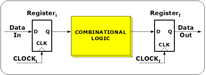
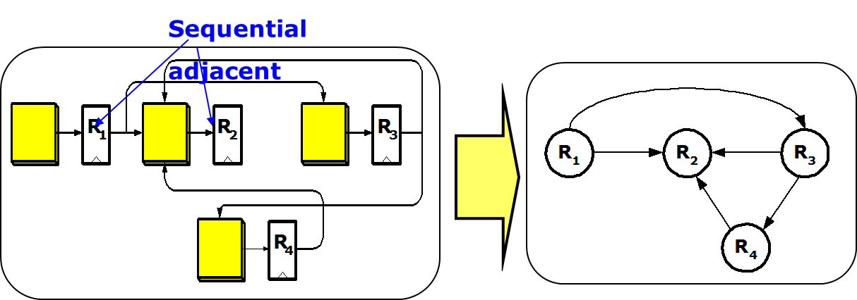
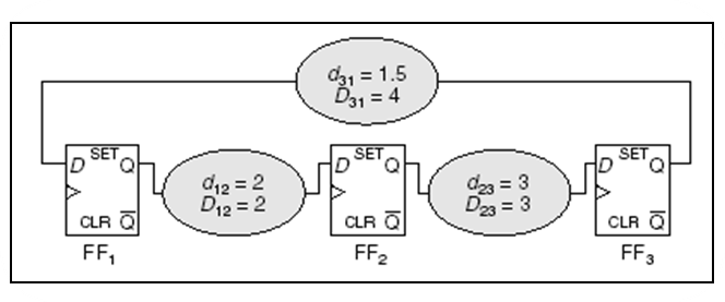
Sequential Logic
-
Local data path
Sequential Logic (cont'd)
-
Graph
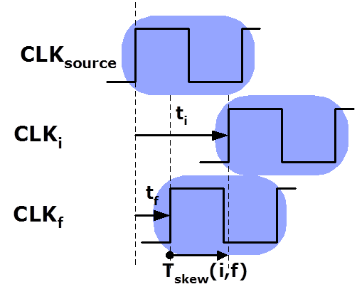
Clock Skew
- , where
- : clock signal delay at the initial register
- : clock signal delay at the final register
Timing Constraint
-
Setup time constraint While this constraint destroyed, cycle time violation (zero clocking) occurs.
-
Hold time constraint While this constraint destroyed, race condition (double clocking) occurs.
Zero skew vs. Useful skew
-
Zero skew () : Relatively easy to implement.
-
Useful skew. Improve:
- The performance of the circuit by permitting a higher maximum clock frequency, or
- The safety margins of the clock skew within the permissible ranges.
-
Max./min. path delays are got from static timing analysis (STA).
Timing Constraint Graph
- Create a graph by
- replacing the hold time constraint with a h-edge with cost from to , and
- replacing the setup time constraint with an s-edge with cost from to .
- Two sets of constraints stemming from clock skew definition:
- The sum of skews for paths having the same starting and ending flip-flop to be the same;
- The sum of clock skews of all cycles to be zero
Timing Constraint Graph (TCG)
Timing Constraint Graph (TCG)
Assume = 0
Clock period is feasible if and only if current graph contains no negative cost cycles.

Minimize Clock Period
-
Linear programming (LP) formulation
where and are sequential adjacent
-
The above constraint condition is so-called system of difference constraints (see Introduction to Algorithms, MIT):
-
👉 Note: easy to check if a feasible solution exists by detecting negative cycle using for example Bellman-Ford algorithm.
Basic Bellman-Ford Algorithm
function BellmanFord(list vertices, list edges, vertex source)
    // Step 1: initialize graph
    for each vertex i in vertices:
        if i is source then u[i] := 0
        else u[i] := inf
        predecessor[i] := null

    // Step 2: relax edges repeatedly
    for i from 1 to size(vertices)-1:
        for each edge (i, j) with weight d in edges:
*           if u[j] > u[i] + d[i,j]:
*               u[j] := u[i] + d[i,j]
*               predecessor[j] := i

    // Step 3: check for negative-weight cycles
    for each edge (i, j) with weight d in edges:
        if u[j] > u[i] + d[i,j]:
            error "Graph contains a negative-weight cycle"
return u[], predecessor[]
Problems with Bellman-Ford Algorithm
- The algorithm is originally used for finding the shortest paths.
- Detecting negative cycle is just a side product of the algorithm.
- The algorithm is simple, but...
- detects negative cycle at the end only.
- has to compute all
d[i,j]. - Restart the initialization with
u[i] := inf. - requests the input graph must have a source node.
Various improvements have been proposed extensively.
Minimize clock period (I)
- Fast algorithm for solving the LP:
- Use binary search method for finding the minimum clock period.
- In each iteration, Bellman-Ford algorithm is called to detect if the timing constraint graph contains negative weighted edge cycle.
- 👉 Note: Originally Bellman-Ford algorithm is used to find a shortest-path of a graph.
Minimize clock period (II)
-
When the optimal clock period is solved, the corresponding skew schedule is got simultaneously.
-
However, many skew values are on the bounds of feasible range.
Yield-driven Clock Skew Scheduling
-
When process variations increase more and more, timing-failure-induced yield loss becomes a significant problem.
-
Yield-driven Clock Skew Scheduling becomes important.
-
Primary goal of this scheduling is to minimize the yield loss instead of minimizing the clock period.
Timing Yield Definition
-
The circuit is called functionally correct if all the setup- and hold-time constraints are satisfied under a group of determinate process parameters.
-
Timing Yield = (functional correct times) / sample number * 100%
Primitive solution (1)
-
Pre-allocate timing margins (usually equivalent to maximum timing uncertainty) at both ends of the FSR's (Feasible Skew Region).
-
Then perform clock period optimization.
Problems with this method
-
The maximum timing uncertainty is too pessimistic. Lose some performance;
-
is fixed; it does not consider data path delay differences between cycle edges.
📑 References (1)
-
"Clock skew optimization", IEEE Trans. Computers, 1990
-
"A graph-theoretic approach to clock skew optimization", ISCAS'94
-
"Cycle time and slack optimization for VLSI-chips", ICCAD'99
-
"Clock scheduling and clocktree construction for high performance Asics", ICCAD'03
-
"ExtensiveSlackBalance: an Approach to Make Front-end Tools Aware of Clock Skew Scheduling", DAC'06
Primitive solution (2)
-
Formulate as LCES (Least Center Error Square) problem
- A simple observation suggests that, to maximize slack, skew values should be chosen as close as possible to the middle points of their FSR's.
📑 References (2)
- Graph-based algorithm
- (J. L. Neves and E. G. Friedman, "Optimal Clock Skew Scheduling Tolerant to Process Variations", DAC'96)
- Quadratic Programming method
- (I. S. Kourtev and E. G. Fredman, "Clock skew scheduling ⏳ for improved reliability via quadratic programming", ICCAD'99)
Shortcoming: might reduce some slacks to be zero to minimum total CES. This is not optimal for yield.
Primitive solution (3)
-
Incremental Slack Distribution
- (Xinjie Wei, Yici CAI and Xianlong Hong, "Clock skew scheduling ⏳ under process variations", ISQED'06)
-
Advantage: check all skew constraints
-
Disadvantage: didn't take the path delay difference into consideration
Minimum Mean Cycle Based
-
Even: solve the slack optimization problem using a minimum mean cycle formulation.
-
Prop: distribute slack along the most timing-critical cycle proportional to path delays
-
FP-Prop: use sensitizable-critical-path search algorithm for clock skew scheduling.
Slack Maximization (EVEN)
-
Slack Maximization Scheduling
-
Equivalent to the so-called minimum mean cycle problem (MMC), where : critical cycle (first negative cycle)
-
Can be solved efficiently by the above method.
Even - iterative slack optimization
-
Identify the circuit's most timing-critical cycle,
-
Distribute the slack along the cycle,
-
Freeze the clock skews on the cycle, and
-
Repeat the process iteratively.
Most timing-critical cycle

Identify the timing-critical cycle
-
Identify the circuit's most timing-critical cycle
-
Solve the minimum mean-weight cycle problem by
- Karp's algorithm
- A. Dasdan and R.K.Gupta, "Faster Maximum and Minimum Mean Cycle Algorithms for System-Performance", TCAD'98.
Distribute the slack
Distribute the slack evenly along the most timing-critical cycle.

Freeze the clock skews (I)
Replace the critical cycle with super vertex.

Freeze the clock skews (II)

To determine the optimal slacks and skews for the rest of the graph, we replace the critical cycle with super vertex.
Repeat the process (I)

Repeat the process (II)

Final result

-
= 0.75
-
= -0.25
-
= -0.5
-
= 1.75
-
= 1.75
-
= 1
where
Problems with Even
- Assume all variances are the same.
- However, the timing uncertainty of a long combinational path is usually larger than that of a shorter path.
- Therefore, the even slack distribution along timing-critical cycles performed by Even is not optimal for yield if data path delays along the cycles are different.
Prop-Based on Gaussian model (I)
- Assuming there are gates with delay in a path, then this path delay is
- Distribute slack along the most timing-critical cycle, according to the square root of each edge's path delays (???).
- To achieve this, update the weights of s-edges and h-edges: where ensures a minimum timing margin for each timing constraint.
Prop-Based on Gaussian model (II)
- Given a specific clock period , we gradually increase and use the Bellman-Ford algorithm to detect whether it is still feasible.
- After finding the maximum , the edges along the most timing-critical cycle will have slacks equal to the pre-allocated timing margins.
- Many edges in a circuit have sufficiently large slack. Therefore, we can perform proportional slack distribution only for the most timing-critical cycle. Assign the rest of skews using Even.
Problems with Prop
- Assume all gate delay has the same distribution.
- Not justify using the square root of path delay for timing margin.
FP-Prop (I)
 : False path
FP-Prop (II)
- If we do not consider false path, some non timing-critical cycles become timing-critical. Then, more slacks are distributed to these cycles, but the slacks in actually timing-critical cycles are not sufficient. As a result, the overall timing yield decreases.
Problems with FP-Prop
- Same problems as Prop
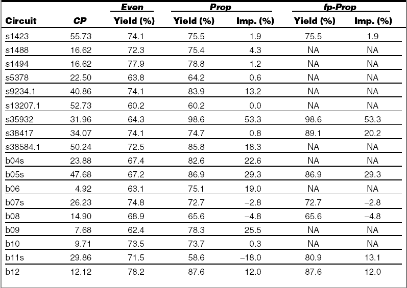
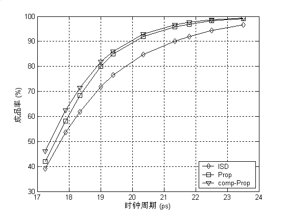
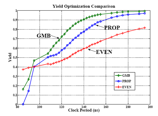
🧪 Experimental Results
📈 Statistical Method
-
Setup time constraint
-
Hold time constraint
where are random variable under process variations.
📈 Statistical TC Graph

After SSTA, edge weight is represented as a pair of value (mean, variance).
Most Critical Cycle
-
Traditional criteria: minimum mean cycle
-
New criteria:
(We show the correctness later)
Slack Maximization (C-PROP)
- Slack Maximization Scheduling
- Equivalent to the minimum cost-to-time ratio problem (MMC), where:
- : critical cycle (first negative cycle)
Probability Observation
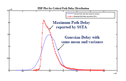
- Prob(timing failure) turns out to be an Error function that solely depends on this ratio. Therefore, it is justified to use this ratio as critical criteria.
Whole flow
-
After determining the clock arrival time at each vertex in the most critical cycle, the cycle is replaced with a super vertex .
-
In-edge from outside vertex to cycle member is replaced by an in-edge with weight mean .
-
Out-edge is replaced by out-edge with weight mean . However, the variance of the edge weight is not changed. And parallel edges can be remained.
-
Repeat the process iteratively until the graph is reduced to a single super vertex, or the edges number is zero.
Data structure

Final result:
Advantages of This Method
- Justified by probability observation.
- Fast algorithm exists for minimum cost-to-time ratio problem.
- Reduce to Even when all variances are equal.
- When a variance tends to zero, it makes sense that only minimal slack is assigned to this variable, and hence others can be assigned more.
Results
📑 Main Reference
- Jeng-Liang Tsai, Dong Hyum Baik, Charlie Chung-Ping Chen, and Kewal K. Saluja, "Yield-Driven, False-Path-Aware Clock Skew Scheduling", IEEE Design & Test of Computers, May-June 2005
Lecture 05b - ⏳ Clock Skew Scheduling Under Process Variations (2)
🗺️ Overview
-
A Review of CSS Issues
-
General Formulation
-
Yield-driven Clock Skew Scheduling
-
Numerical Results
Minimum Clock Period Problem
-
Linear programming (LP) formulation
where and are sequentially adjacent to each other.
-
The above constraints are called system of difference constraints (see Introduction to Algorithms, MIT):
- Key: it is easy to check if a feasible solution exists by detecting negative cycles using the Bellman-Ford algorithm.
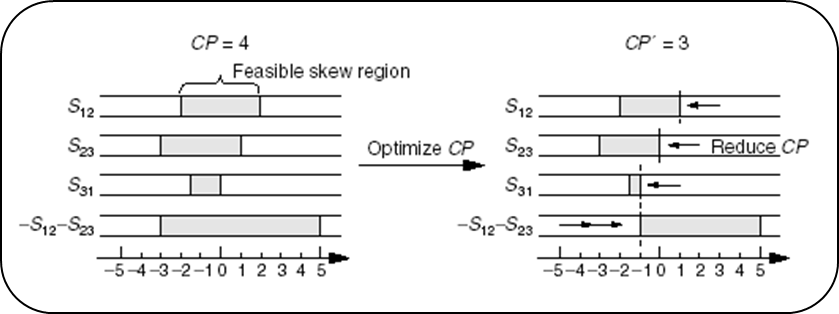
System of Difference Constraints
- In some cases, you may need to do some transformations, e.g.
Slack Maximization (EVEN)
-
Slack Maximization Scheduling
(👉 Note: )
-
is equivalent to the so-called minimum mean cycle problem (MMC), where:
- ,
- : critical cycle (first negative cycle)
-
Can be efficiently solved by the parametric shortest path methods.
Slack Maximization (C-PROP)
-
Slack Maximization Scheduling
(we show the correctness later)
-
is equivalent to the minimum cost-to-time ratio problem (MCR), where:
- ,
- : critical cycle
General Formulation
- General form: where a linear function that represents various problems defined above.
| Problem | (setup) | (hold) | |
|---|---|---|---|
| Min. CP | |||
| EVEN | |||
| C-PROP |
General Formulation (cont'd)
-
In fact, and are not necessarily linear functions. Any monotonic decreasing function will do.
-
Theorem: if and are monotonic decreasing functions for all and , then there is a unique solution to the problem. (prove later).
-
Question 1: Does this generalization have any application?
-
Question 2: What if and are convex but not monotone?
🔕 Non-Gaussian Distribution
-
65nm and below, the path delay is likely to have a non-Gaussian distribution:
👉 Note: central limit theorem does not apply because
- random variables are correlated (why?)
- delays are non-negative
Timing Yield Maximization
-
Formulation:
- is not exactly timing yield but reasonable.
-
It is equivalent to:
where
-
Luckily, any CDF must be a monotonic increasing function.
📈 Statistical Interpretations of C-PROP
-
Reduce to C-PROP when is Gaussian, or precisely
-
EVEN: identical distribution up to shifting
Not necessarily worse than C-PROP
⚖️ Comparison
Three Solving Methods in General
- Binary search based
- Local convergence is slow.
- Cycle based
- Idea: if a solution is infeasible, there exists a negative cycle which can always be "zero-out" with minimum effort (proof of optimality)
- Path based
- Idea: if a solution is feasible, there exists a (shortest) path from where we can always improve the solution.
Parametric Shortest Path Algorithms
-
Lawler's algorithm (binary search)
-
Howard's algorithm (based on cycle cancellation)
-
Hybrid method
-
Improved Howard's algorithm
-
Input:
- Interval [tmin, tmax] that includes t*
- Tol: tolerance
- G(V, E): timing graph
-
Output:
- Optimal t* and its corresponding critical cycle C
Lawler's Algorithm
@startuml
 while ((tmax - tmin) > tol)
    : t := (tmin + tmax) / 2;
    if (a neg. cycle C under t exists) then
       : tmax := t;
    else
       : tmin := t;
    endif
 endwhile
 : t* := t;
@enduml
Howard's Algorithm
@startuml
 : t := tmax;
 while (a neg. cycle C under t exists)
    : find t' such that
      sum{(i,j) in C | fij(t')} = 0;
    : t := t';
 endwhile
 : t* := t;
@enduml
Hybrid Method
@startuml
 while ((tmax - tmin) > tol)
    : t := (tmin + tmax) / 2;
    if (a neg. cycle C under t exists) then
       : find t' such that
         sum{(i,j) in C | fij(t')} = 0;
       : t := t';
       : tmax := t;
    else
       : tmin := t;
    endif
 endwhile
 : t* := t;
@enduml
Improved Howard's Algorithm
@startuml
 : t := (tmin + tmax) / 2;
 while (no neg. cycle under t)
    : tmin := t;
    : t := (tmin + tmax) / 2;
 endwhile
 while (a neg. cycle C under t exists)
    : find t' such that
      sum{(i,j) in C | fij(t')} = 0;
    : t := t';
 endwhile
 : t* := t;
@enduml
]
⏳ Clock Skew Scheduling for Unimodal Distributed Delay Models
@luk036
2022-10-26
Useful Skew Design: Why and Why not?
Bad 👎:
- Needs more engineer training.
- Balanced clock-trees are harder to build.
- Don't know how to handle process variation, multi-corner multi-mode, ..., etc.
Good 👍:
If you do it right,
- spend less time struggling about timing, or
- get better chip performance or yield.
What can modern STA tools do today?
- Manually assign clock arrival times to registers (all zeros by default)
- Grouping: Non-critical parts can be grouped as a single unit. In other words, there is no need for full-chip optimization.
- Takes care of multi-cycle paths, slew rate, clock-gating, false paths etc. All we need are the reported slacks.
- Provide 3-sigma statistics for slacks/path delays (POCV).
- However, the full probability density function and correlation information are not available.
Unimodality
-
In statistics, a unimodal probability distribution or unimodal distribution is a probability distribution with a single peak.
-
In continuous distributions, unimodality can be defined through the behavior of the cumulative distribution function (cdf). If the cdf is convex for and concave for , then the distribution is unimodal, being the mode.
-
Examples
- Normal distribution
- Log-normal distribution
- Log-logistic distribution
- Weibull distribution
Quantile function
-
The quantile function of a distribution is the inverse of the cumulative distribution function .
-
Close-form expression for some unimodal distributions:
- Normal:
- Log-normal:
- Log-logistic:
- Weibull:
-
For log-normal distribution:
- mode:
- CDF at mode:
Normal vs. Log-normal Delay Model
Normal/Gaussian:
- Convertible to a linear network optimization problem.
- Supported over the whole real line. Negative delays are possible.
- Symmetric, obviously not adaptable to the 3-sigma results.
Log-normal:
- Non-linear, but still can be solved efficiently with network optimization.
- Supported only on the positive side.
- Non-symmetric, may be able to fit into the 3-sigma results. (???)
Setup- and Hold-time Constraints
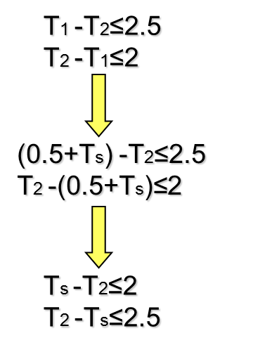
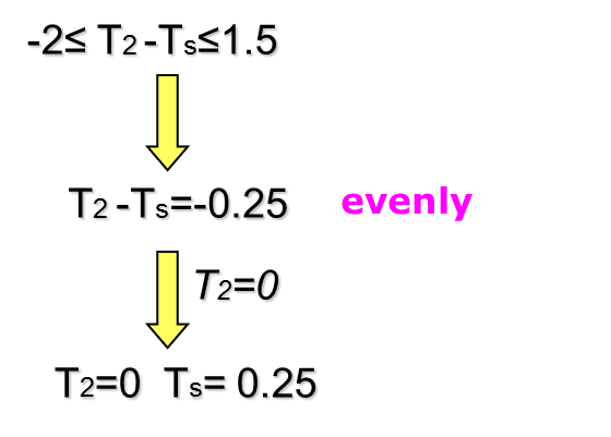
- Let , where
- : clock signal delay at the initial register
- : clock signal delay at the final register
- Assume in zero-skew, i.e. , the reported setup- and hold-time slacks are _ and _ respectively.
- Then, in useful skew design:
- In principle, represent the minimum- and maximum-path delay, and should be always greater than zero.
- Let
Yield-driven Optimization
- Max-Min Formulation:
- ,
- No need for correlation information between paths.
- Not exactly the timing yield objective but reasonable.
- Equivalent to:
- or:
Yield-driven Optimization (cont'd)
- In general, Lawler's algorithm (binary search) can be used.
- Depending on the distribution, there are several other ways to solve problem.
Gaussian Delay Model
- Reduce to:
- Linearization. Since is anti-symmetric and monotonic, we have:
-
is equivalent to the minimum cost-to-time ratio (linear).
-
However, actual path delay distributions are non-Gaussian.
Log-normal Delay Model
- Reduce to:
- Since is anti-symmetric and monotonic, we have:
- Bypass evaluating error function. Non-linear and non-convex, but still can be solved efficiently by for example binary search on .
Weibull Delay Model
- Reduce to: